6.5 Assessment of the impact of investment projects on the development of the city
In 2020, by order of a major development institution, the Digital Twin (DT) team developed and automated a methodology for assessing the impact of investment projects on the socio-economic development (SED) of cities. The results of this work are intended to form optimal investment portfolios for infrastructure development based on their contribution to city development.
6.5.1 Purpose of the methodology
The methodology defines: - A set of socio-economic development (SED) indicators for cities; - The procedure for collecting and processing statistical data on SED indicator values; - The procedure for assessing the contribution of SED indicators to achieving national goals; - The procedure for forming a baseline (inertial) SED forecast reflecting current trends and factors; - A method for assessing the magnitude of mutual influence between SED indicators and their susceptibility to changes in external factors; - The procedure for assessing and ranking investment potentials of cities by economic activity and territory; - The procedure for assessing the impact of an investment project on SED.
Main principles of the Methodology: - Ensuring a unified approach to quantitative and comparative assessment of the achieved and forecasted level of socio-economic development of cities, identifying and comparing their potentials between different cities, and assessing the impact of external factors and investment projects over a long-term period; - Identifying and ranking investment niches and projects aimed at achieving maximum effects while maintaining a balance of economic interests of the city, the bank, and the project operator; - Assessing multiplicative and dynamic effects of an intersectoral, interterritorial, and inter-species nature; - Identifying implicit links and conditions for obtaining the maximum effect from investments; - Solving forecasting and impact assessment problems.
6.5.2 Normative references and literature
- Decree of the President of the Russian Federation of 07.05.2018 No. 204 “On national goals and strategic tasks of development of the Russian Federation for the period until 2024”.
- Federal Law “On Strategic Planning in the Russian Federation” of 28.06.2014 No. 172-FZ.
- Decree of the Government of the Russian Federation of 13.02.2019 No. 207-r on the approval of the Spatial Development Strategy of the Russian Federation.
- Fundamentals of the state policy of regional development of the Russian Federation for the period until 2025 (approved by the Decree of the President of the Russian Federation on 16.01.2017 No. 13).
- Decree of the Government of 27.12.2019 No. 3227-r on the approval of the Implementation Plan for the Spatial Development Strategy of the Russian Federation.
- Forecast of socio-economic development of the Russian Federation for the period until 2036 (approved at a meeting of the Government of the Russian Federation on 22.11.2018).
- Order of the Ministry of Economic Development of the Russian Federation of March 27, 2019, No. 167 “On the approval of the form of the test-passport of the capital construction object and the Methodology for assessing the effectiveness of the use of federal budget funds directed for capital investments”.
- Decrees of the Government of the Russian Federation No. 510-r of March 23, 2019, “On the approval of the methodology for assessing the quality of the urban environment”.
- Resolution of the Government of 29.11.2019 No. 1512 “On the approval of the methodology for assessing socio-economic effects from construction (reconstruction) and operation projects of transport infrastructure objects planned for implementation with the involvement of federal budget funds, as well as with the provision of state guarantees of the Russian Federation and tax benefits”.
- Order of the Ministry of Economic Development of Russia of 14.12.2013 No. 741 “On the approval of methodological guidelines for the preparation of strategic and complex justifications of the investment project, as well as for the assessment of investment projects claiming financing from the National Wealth Fund and (or) pension savings under the trust management of the state management company, on a returnable basis”.
- System of National Accounts 2008. Statistical framework: a comprehensive, systematic, and flexible set of macroeconomic accounts used for policy development, analysis, and research. United Nations, World Bank, Organization for Economic Cooperation and Development.
- S. P. Kapitsa. Paradoxes of Growth: Laws of Human Development. - M.: “Alpina Non-fiction”, 2010. p. 192. - ISBN 978-5-9167-1047-2.
- Jay Forrester. “Urban Dynamics”. 1974.
- Wassily Leontief. “Input-Output Economics”. 1997.
6.5.3 Terms and Definitions
Baseline indicators — quantitatively measurable indicators for which statistical, sociological observations or direct measurements are possible.
Baseline forecast (inertial scenario) — a set of values for city socio-economic development indicators for a prospective period, assuming the preservation of established trends.
Business type — a type of economic activity aimed at making a profit.
G(R)DP — Gross (Regional) Domestic Product.
Boundary conditions — maximum and minimum values that a particular indicator can take according to calculations performed in the mathematical model.
Assumptions on external factors — scenario values of parameters used for building forecasts.
Dimension — an attribute of an indicator containing a numerical value or a set of numerical values characterizing one of the representations of an object (process, function) or its decomposition.
Investment potential — calculated volume of investment, the return of which is possible due to additional profit in individual types of economic activity by increasing sales and improving economic efficiency of production, as well as increasing the level of provision with socio-economic objects.
Integral assessment of sectoral market niches — assessment of the investment potential for a particular type of economic activity in a particular city, with possible spatial referencing.
Methodology — Methodology for assessing the impact of an investment project on the socio-economic development of the city.
Module (software module) — a functionally complete fragment of a program, designed as a separate file(s) with source code or a named continuous part of it, intended for use in the system.
Set of provisions — the result of development in the form of mathematical, methodological, and informational provisions.
Direction (sphere, industry) of city economy — an industry (sphere, type of economic activity) of the city economy to which the Methodology can be applied.
Provision with SEO — an indicator characterizing the quality of the urban environment through the level of satisfaction of the population’s needs for socio-economic objects (SEO) according to urban planning standards.
Assessment of the impact of an investment project on SED — change in the indicators of the scenario and baseline versions of the SED forecast in absolute and relative indicators as a result of the implementation of the IP.
Investment project configuration parameters — numerical values of financial, sectoral, and other indicators of the project, reflected in the form of a completed Investment Project Passport.
City Passport — a form for collecting and presenting values of socio-economic development indicators and individual spheres of the city economy.
Investment Project Passport — a form for collecting and presenting characteristics of an investment project.
Population density — the number of residents (population) per unit area of the territory.
Indicator — a numerical value or a set of numerical values characterizing the state of an object (process, function).
Industrial business types — business types involving the production of industrial products, consumption of which is carried out both within the region where the production enterprise is located and in other constituent entities of the Russian Federation.
Calculation modules — modules consisting of input, calculation, and output forms (indicators) that implement individual functions of calculation, analysis, and assessment described in the Methodology.
Region — a constituent entity of the Russian Federation.
Service business types — business types in the sphere of city commercial retail services, including industries such as retail trade, public catering, leisure and entertainment, education, and healthcare.
Scenario — one of the variants of the city’s SED with given forecasting parameters regarding external factors.
Scenario forecast — development of the city taking into account the implementation of an investment project.
Data warehouse — an information subsystem providing storage and updating of data in a specific structure required for conducting analytical research or mathematical calculations.
Target city — a city (municipality) of the Russian Federation for which it is possible to obtain the necessary data for the initial filling of the system.
Target indicators — indicators including indicators of national goals and national projects of the Russian Federation.
Target sales region — a region from which revenue from the sale of products covers the costs of production, sale, and transportation of products manufactured in the target city.
6.5.4 Symbols, Abbreviations, and Data Sources
6.5.4.1 Sources of Input Data
| No. | Source of Information |
|---|---|
| S1 | Balance Sheets |
| S2 | Fixed Assets |
| S3 | SNA Data |
| S4 | SNA Methodology |
| S5 | Input-Output Methodology |
| S6 | All-Russian Classifier of Territories of Municipal Formations (OKTMO) |
| S7 | All-Russian Classifier of Types of Economic Activity (OKVED) |
| S8 | Municipal Statistics |
| S9 | Regional (Municipal) Urban Planning Standards |
| S10 | Investment Project Passport. Appendix. Document Code DT.0427 |
| S11 | Aggregated Cost Standards (NTS-81-02-XX-2020) |
| S12 | Average Annual Production Capacity |
| S13 | Areas of Socio-Economic Objects (GIS) |
6.5.4.2 Abbreviations
GCP — Gross City Product.
IP — Investment Project.
SME — Small and Medium-sized Enterprises.
SEO — Socio-Economic Objects.
SED — Socio-Economic Development.
RF — Russian Federation.
PF — Payroll Funds.
B2C — Business to customer (final consumption by households).
B2B — Business to business (final and intermediate consumption by non-households).
6.5.4.3 Symbols
Indices:
| No. | Indicator Name | Symbol | Data Source |
|---|---|---|---|
| 1 | Time (calendar date), year - superscript index | \(^{t}\) | - |
| 2 | Base year - superscript index | \(^{b}\) | - |
| 3 | Industry number - subscript index | \(_{i}\) | S5 |
| 4 | City number - subscript index | \(_{j}\) | S6 |
| 5 | Russian Federation - subscript index | \(_{fed}\) | - |
| 6 | Constituent entity of the Russian Federation - subscript index | \(_{reg}\) | - |
Demographic indicators:
| No. | Indicator Name | Symbol | Data Source |
|---|---|---|---|
| 7 | Population, people | \(N\) | S8 |
| 8 | Number of births, people | \(B\) | S8 |
| 9 | Number of deaths, people | \(D\) | S8 |
| 10 | Number of arrivals for permanent residence, people | \(I\) | S8 |
| 11 | Number of departures for permanent residence, people | \(O\) | S8 |
| 12 | Natural increase (decrease), people | \(N_{e}\) | S8 |
| 13 | Migration increase (decrease), people | \(N_{m}\) | S8 |
| 14 | Population younger than working age, people | \(N_{y}\) | S8 |
| 15 | Working-age population, people | \(N_{w}\) | S8 |
| 16 | Population older than working age, people | \(N_{s}\) | S8 |
| 17 | Average number of employees of organizations, people | \(N_{z}\) | S8 |
| 18 | Growth rate of life expectancy, % | \(T_{le}\) | Formula 6.1 |
Economic indicators (in rubles):
| No. | Indicator Name | Symbol | Data Source |
|---|---|---|---|
| 19 | Capital of organizations | \(K\) | S1 |
| 20 | Reserve capital of organizations | \(K_{r}\) | S1 |
| 21 | Long-term liabilities of organizations | \(K_{l}\) | S1 |
| 22 | Inventories of organizations | \(K_{z}\) | S1 |
| 23 | Balance of organizations | \(BB\) | S1 |
| 24 | Average annual cost of fixed assets, rub. | \(F_{A}\) | S1 |
| 25 | Own working capital | \(F_{O}\) | Formula (37.1) |
| 26 | Current assets, rub. | \(F_{L}\) | S8 |
| 27 | Gross Domestic Product (Gross City Product), rub. | \(GDP\) | Formula (1) |
| 28 | Revenue, rub. | \(R\) | S1 |
| 29 | Gross Value Added, rub. | \(GVA\) | S1 |
| 30 | Payroll of all employees of organizations, rub. | \(S\) | S8 |
| 31 | Average monthly salary of employees of organizations, rub. | \(S_{M}\) | S8 |
| 32 | Non-taxable income of the population, rub. | \(S_{C}\) | Formula (4) |
| 33 | Social and other payments, rub. | \(S_{P}\) | S8 |
| 34 | Consumption of fixed capital (depreciation), rub. | \(A\) | Formula (3) |
| 35 | Taxes less other subsidies on production, rub. | \(T_{P}\) | S1 |
| 36 | Taxes less subsidies on products - indirect taxes, rub. | \(T_{K}\) | Formula (2) |
| 37 | Profit before tax, thousand rubles | \(P_{d}\) | S1 |
| 38 | Net profit (net mixed income), rub. | \(P_{n}\) | S1 |
| 39 | Unit output matrices, share | \(e\) | S3 |
| 40 | Unit consumption matrices, share | \(a_{rf}\) | S3 |
| 41 | Sectoral proportion, share | \(P\) | S3 |
| 42 | Population income, rub. | \(R_{H}\) | Formula (9) |
| 43 | Real disposable income of citizens, rub. | \(P_{g}\) | Formula (8) |
| 44 | Mandatory expenses of the population, rub. | \(L_{H}\) | Formula (10) |
| 45 | Cost of sales, rub. | \(L_{P}\) | S1 |
| 46 | Commercial expenses, rub. | \(L_{C}\) | S1 |
| 47 | Management expenses, rub. | \(L_{U}\) | S1 |
| 48 | Payments to suppliers (contractors) for raw materials, materials, works, services (For the reporting year), rub. | \(L_{M}\) | S1 |
| 49 | Payments in connection with labor remuneration of employees (For the reporting year), rub. | \(L_{T}\) | S1 |
| 50 | Trade and transport margins, rub. | \(L_{TT}\) | S3 |
| 51 | Insurance payments, rub. | \(L_{S}\) | Formula (22) |
| 52 | Capital investments, rub. | \(L_{Ci}\) | S8 |
| 53 | Import, rub. | \(Im\) | |
| 54 | Production capacity, unit/year | \(Q_{i}^{*}\) | S12 |
Indicators of provision with socio-economic objects:
| No. | Indicator Name | Symbol | Data Source |
|---|---|---|---|
| 55 | Total area of residential premises, sq. m | \(P\) | S8 |
| 56 | Capacity of SEO objects, unit | \(Q_{k}^{*}\) | S10 |
| 57 | Regional provision standards by type of SEO objects, unit/person | \(Q_{H}\) | S9 |
| 58 | Type of SEO objects | \(k\) | section 6.5. |
| 59 | Volume of final demand for products, rub. | \(Y\) | Formula (17) |
Generalizing indicators:
| No. | Indicator Name | Symbol | Data Source |
|---|---|---|---|
| 60 | Investment potential, rub. | \(L^{*}\) | Formula (27) |
| 61 | Normative payback period of capital investments, years | \(T^{*}\) | Set by specialist |
| 62 | Profitability of production, rub./rub. | \(E_{F}\) | Formula (32) |
| 63 | Labor productivity, rub./person | \(E_{T}\) | Formula (21) |
| 64 | Efficiency of material resource use, rub./rub. | \(E_{M}\) | Formula (23) |
| 65 | Efficiency of using working capital (profitability of working capital), rub./rub. | \(E_{FL}\) | Formula (18) |
| 66 | Efficiency of using non-current (fixed) assets, asset turnover, rub./rub. | \(E_{FA}\) | Formula (20) |
| 67 | Specific available capacity of SEO per capita, unit/person | \(E_{k}\) | Formula (29) |
| 68 | Provision with SEO objects, % | \(O\) | Formula (16) |
| 69 | Housing provision, sq. m/person | \(O_{h}\) | Formula (11) |
| 70 | Industry resistance to negative external factors | \(U_{i}\) | Formula (34) |
| 71 | Target indicators | \(KPI\) | Formulas (5), (6), (7), (11), (14) |
| 72 | Multiplier matrix | \(b\) | Formula (38.1) |
| 73 | Net Present Value | \(NPV\) | Formula (40) |
| 74 | Internal Rate of Return | \(IRR\) | Formula (41) |
| 75 | Payback period of capital investments | \(PP\) | Formula (42) |
| 76 | Financial independence of organizations | \(F_{i}\) | Formula (35) |
| 77 | Financial stability of organizations | \(F_{s}\) | Formula (36) |
| 78 | Financial maneuverability of organizations | \(F_{m}\) | Formula (37) |
| 79 | Provision with current assets of organizations | \(F_{F}\) | Formula (38) |
| 80 | Provision with inventories | \(F_{Z}\) | Formula (39) |
Relative or unit indicators (coefficients):
| No. | Indicator Name | Symbol | Data Source |
|---|---|---|---|
| 81 | Unit capital investments for the construction of a unit of SEO capacity | \(I_{k}\) | S11 |
| 82 | Unit volume of gross value added | \(gva\) | Formula (31) |
Investment project indicators:
| No. | Indicator Name | Symbol | Data Source |
|---|---|---|---|
| 83 | Investment project number - subscript index | \(z\) | - |
| 84 | Project life cycle duration | \(T_{z}\) | S10 |
| 85 | Project costs | \(L_{z}\) | S10 |
| 86 | Discount rate | \(d\) | S10 |
6.5.5 General Provisions
- The methodology defines a set of baseline and target indicators characterizing three aspects of the city’s SED:
- demography (population size and derivative parameters);
- economy (gross city product and its components);
- provision with SEO objects.
- Baseline demographic indicators include:
- population size;
- natural increase (number of births and deaths);
- migration increase (number of arrivals and departures for permanent residence).
Demographic indicators are grouped by age structure.
- Baseline economic indicators include:
- gross domestic (city) product;
- income and mandatory expenses of the population;
- revenue, costs, and profit of enterprises;
- income and expenses of budgets of all levels;
- accumulation and consumption of fixed capital.
Economic indicators are grouped: - by type of economic activity according to OKVED (with possible isolation of SMEs); - by the structure of balance sheet indicators (assets and liabilities, income and expenses, receipts and payments).
- Baseline indicators of provision with socio-economic objects include:
- total area of residential premises;
- housing completion rates;
- provision with socio-economic objects.
- Indicators of provision with socio-economic objects are grouped by type of socio-economic object:
- education (preschool educational organizations, general educational organizations);
- healthcare (number of hospital beds, capacity of outpatient clinics);
- trade (retail space);
- culture (libraries, cinemas, theaters, club-type cultural institutions, culture and leisure parks);
- sports (gyms, outdoor sports facilities, swimming pools).
- The list of baseline indicators of city socio-economic development is used to calculate target indicators of socio-economic development of the city and the Russian Federation. Based on retrospective statistics, the values of baseline indicators are determined in physical1 and monetary terms, which are further used to form baseline (inertial) and scenario (investment) variants of the forecast of the city’s socio-economic development.
Target indicators of socio-economic development of the Russian Federation include indicators of national goals and national projects of the Russian Federation.
Target indicators of the demographic aspect of city socio-economic development include:
- population growth, in number of people;
- life expectancy, in number of years.
- Target indicators of the economic aspect of city socio-economic development include:
- population size,
- life expectancy,
- working-age population,
- profit (loss) of enterprises and organizations from sales,
- gross city product,
- income of small and medium-sized enterprises (SMEs),
- local budget revenues (tax),
- fixed assets of enterprises,
- real disposable income of the population,
- labor productivity,
- employment of the population,
- housing provision.
- Target indicators of provision with socio-economic objects include:
- housing provision for the population, in square meters per capita;
- urban environment quality index, measured in percent.
To form an assessment of the current state of the city, the sources of input data indicated above are used.
The methodology defines a list of indicators and parameters characterizing the investment project necessary for conducting an assessment of its impact on the city’s SED.
The methodology includes recommendations for the analysis and assessment of effects from the implementation of investment projects in the sphere of the city economy, including:
- recommendations for identifying and assessing investment potentials in cities;
- recommendations for assessing the economic efficiency of the IP;
- recommendations for assessing the impact of the IP on the city’s SED;
- recommendations for methods of SED analysis;
- recommendations for methods of analysis and generalizations of scenario variants of city SED indicator forecasts;
- recommendations for configuring assumptions (assumptions on external factors) for forming baseline and scenario variants of forecasts.
- The methodology includes a sequence of actions (assessment algorithm) for:
- Assessing the current and forecasted state of city development.
- Integral assessment of the investment potential of cities.
- Assessing the investment attractiveness of target directions (industries) of the city economy.
- Assessing and ranking cities for each target direction (industry) of the city economy.
- Assessing the effectiveness of the investment project implementation and its impact on the forecasted indicators of the city’s SED.
6.5.6 Assessing the Current and Forecasted State of City Development
Assessment of the current and forecasted state of the city’s SED is performed based on retrospective values of baseline indicators formed in the “City Passport”.
At the stage of assessing the current and forecasted state of the city’s SED, the following are calculated:
- Actual values of the gross city product.
- Contribution of the city to achieving national goals.2
- Baseline (inertial) scenario of the city’s SED for a prospective horizon until 2040.
- Mutual correlation of socio-economic development indicators throughout the planning horizon until 2040.
- Calculation of actual values of the gross city product is performed by summing the volumes of payroll funds, net profit of enterprises, accrued taxes3, consumption of fixed capital (depreciation), and non-taxable income of the population (based on the volume of taxable income of the population and individual entrepreneurs).
Gross City Product:
\[ GDP=(S+S_{c})+A+P_{n}+(T_{p}+T_{k}), \ \ (1) \]
where the amount of indirect taxes generated by the city is:
\[ T_{k}=\frac{NB_{fed}}{R_{fed}}*R, \ \ (2) \]
where depreciation of fixed assets in the city is:
\[ A=\frac{A_{fed}}{FA_{fed}}*FA, \ \ (3) \]
where the assessment of the magnitude of non-taxable income of the population (“gray” wages) is:
\[ S_{c}=(N_{w}-N_{z}) * S_{M} * 12 \ \ (4) \]
- Calculation of the city’s contribution to achieving national goals (\(KPI\)) is performed for the following target indicators:
4.1. Growth rate of the gross city product:
\[ \dot{GDP}=GDP^{t}/GDP^{t-1} \ \ (5) \]
where \(GDP^{t}\) is the value of the gross domestic (city) product for year t.
4.2. Natural population increase:
\[ E=B-D \ \ (6) \]
4.3. Increase in life expectancy (absolute, years):
\[ T_{le}=N^{t}/D^{t}-N^{t-1}/D^{t-1} \ \ (6.1) \]
4.4. Growth of real disposable income of the population:
\[ \begin{aligned} &\dot{P_{h}}=P_{h}^{t}/P_{h}^{t-1} \ \ &(7)\\ &P_{h}=R_{H}-L_{H} \ \ &(8)\\ &R_{H}=S+S_{C}+S_{P} \ \ &(9)\\ &L_{H}=N*L_{H}^{reg}/N^{reg} \ \ &(10) \end{aligned} \]
where the index \(^{reg}\) denotes the value of the indicator for the region where the city is located.
4.5. Improvement of housing conditions through the increase in housing provision:
\[ \begin{aligned} &\dot{O_{h}}=O_{h}^{t}/O_{h}^{t-1} \ \ &(11)\\ &O_{h}=P_{h}/N \ \ &(12) \end{aligned} \]
- Calculation of the city’s achievement of national goals for indicators having values in physical or monetary units of measurement (GCP, population size, natural population increase, increase in real disposable income) is produced proportionally to the share of this city in the Russian Federation by the population size parameter.
\[ IN=\frac{KPI}{KPI_{RF}*N/N_{RF}} \ \ (13) \]
- Calculation of the city’s achievement of national goals for indicators having values in percent (growth rates, labor productivity, employment) is produced by the following formula:
\[ IN=KPI/KPI_{RF} \ \ (13.1) \]
- Calculation of target indicators of the city’s SEO provision is produced for individual types of economic activity and types of socio-economic objects (the list is given in section 6.5) by the following formula:
\[ O=\sum O_{i}/KI \ \ (14) \]
where \(KI\) is the number of types of economic activity of a social nature,
\[ O_{i}=\sum O_{k}/KK \ \ (15) \]
where \(KK\) is the number of types of SEO objects,
\[ \begin{aligned} & O_{k}=Q_{k}^{*}/Y_{k} \ \ &(16)\\ & Y_{k}=N*Q_{H} \ \ &(17) \end{aligned} \]
- The calculation of the baseline (inertial) scenario of the city’s SED for a prospective horizon until 2040, as well as missing values of baseline indicators for the retrospective period, are formed on the basis of input retrospective data formed in the City Passport. The calculation of these indicators is performed using approximating and dynamic functions in 5 stages of forecasting:
- Formation of forecast corridors for demographic indicators.
- Distribution of demographic indicators by age groups.
- Formation of forecast corridors for economic indicators.
- Formation of a dynamic forecast of demographic and economic indicators.
- Calculation of target indicators for the forecast period.
- At the first stage of forecasting, forecast corridors (constraints) are formed by the least squares method, determining long-term trends (approximating function) of population growth according to the scientific-methodological approach of Academician of the RAS S.P. Kapitsa.
- Input data and forecasted demographic indicators are population size, birth rate, mortality, migration arrival, and departure of the population from the city. Forecast values for demographic indicators are determined by calculating the values of the approximating function by year.
- Forecast values for demographic indicators are used to determine forecast values for economic indicators and indicators of provision with socio-economic objects, including:
- housing provision for the population with socio-economic objects (the ratio of actual SEO capacity to the standardized local or regional demand for SEO services);
- volumes of final product consumption in the sphere of the city economy.
- At the second stage of forecasting, population size indicators are divided into 3 components according to the actual proportion: working-age population, population younger than working age, and population older than working age.
- To calculate the provision of children with education facilities, the indicator of the population younger than working age is used.
- Population size indicators older than working age are used for assessing the size of social payments (participating in the assessment of population income).
- To calculate non-taxable income of the population, working-age population indicators are used, less the average number of jobs.
- Working-age population indicators are used to determine available labor resources in the city’s territory.
- At the third stage of forecasting, forecast corridors (constraints) are formed by the maximum likelihood method, based on statistical series, determining long-term trends (approximating function) of changes in the following economic indicators4:
- gross city product;
- local taxes and local budget expenses;
- average size of pension accruals;
- revenue, costs, and profit of enterprises;
- total residential premises, housing completions;
- payroll funds, average wages, average number of employees;
- taxable monetary income of individuals and individual entrepreneurs, population income, and other payments;
- enterprise revenue, enterprise costs (at the established level of profitability).
- At the fourth stage, a dynamic forecast of baseline SED indicators is formed, limited by the corridor of forecast values determined at the previous forecasting stages.
The methodological basis for forming this forecast is the city system dynamics model (“Urban dynamics”), developed by J.W. Forrester.
According to this model, a dynamic forecast of the behavior of individual SED indicators is initially calculated: - city population; - gross city product; - fixed capital investment; - average number of employees of organizations; - working-age population; - local budget revenues (tax revenues); - local budget expenses; - payroll of all employees of organizations; - taxable monetary income of individuals and individual entrepreneurs; - population income (social and other payments); - enterprise revenue; - profit (loss) from sales of enterprises; - fixed assets of enterprises; - real disposable income of the population; - volume of working capital; - volume of non-current (fixed) assets; - housing completions; - total area of residential premises; - SEO provision.
To determine the dynamic behavior of individual city spheres, a system of second-order differential equations (dynamic function) is used, describing the behavior of the system under the influence of a complex of external factors and its own oscillation and damping characteristics.
The parameters (relative coefficients) of the dynamic function are selected by the least squares method within the value corridors set by the approximating functions developed at the stages described in points 7.8, 7.10.
Based on the obtained parameters, missing and “anomalous” values in retrospective series, as well as forecast values of baseline SED indicators, are calculated.
The general forecasting flow chart is presented in the figure.
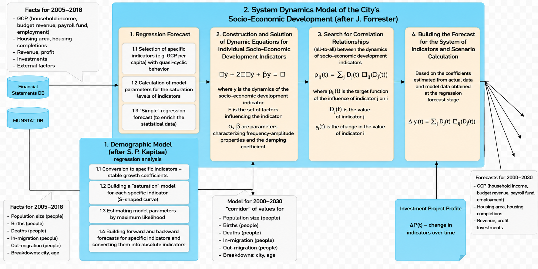
At the fifth stage of forecasting, target indicators for the forecast period are calculated according to formulas (1)-(17).
Based on the calculated dynamic function for SED indicators, correlation functions are calculated, describing the measure of mutual influence of indicators on each other and susceptibility to changes in external factors.
Correlation functions are used for calculating the degree of susceptibility of SED indicators over time to changes in SED indicators caused by the parameters of the implemented investment project.
The parameters of the correlation function are recorded in a correlation (square) matrix of dimension 31 by 31 (by the number of baseline socio-economic indicators), where a quantitative measure of the mutual influence of indicator changes is recorded in the cells. The correlation matrix further participates in the calculation of system-dynamic effects from the implementation of the investment project.
Indicators included in the 31 x 31 correlation matrix:
| No. | Code | Indicator | Unit |
|---|---|---|---|
| 1 | C013 | Population as of January 1 of the current year | people |
| 2 | C034 | Number of births | people |
| 3 | C035 | Number of deaths | people |
| 4 | C037 | Population inflow (migration) | people |
| 5 | C038 | Population outflow (migration) | people |
| 6 | C041 | Working-age population | people |
| 7 | C096 | Completion of apartment buildings | \(m^{2}\) |
| 8 | C149 | Total area of residential premises | \(m^{2}\) |
| 9 | C221 | Average number of employees of organizations, total | people |
| 10 | C241 | Payroll of all employees of organizations, total | rubles |
| 11 | C698 | Taxable monetary income of individuals and individual entrepreneurs | rubles |
| 12 | C699 | Population income: social and other payments | rubles |
| 13 | C712 | Monetary income per capita | rub. per year |
| 14 | C713 | Mandatory payments and contributions per capita | rub. per year |
| 15 | C714 | Real disposable income per capita | rub. per year |
| 16 | C757 | Integral SEO provision for the city | % |
| 17 | C049 | City budget revenues, total | mln. rub. |
| 18 | C065 | City budget expenses, total | mln. rub. |
| 19 | C087 | Fixed capital investment by organizations (excluding small business) | mln. rub. |
| 20 | C706 | Gross City Product (GCP) | mln. rub. |
| 21 | C708 | Tax revenues of budgets of all levels | mln. rub. |
| 22 | C709 | Local budget revenues (tax) | mln. rub. |
| 23 | C433 | Current assets | mln. rub. |
| 24 | C475 | Revenue (For the reporting period) | mln. rub. |
| 25 | C711 | Total cost (revenue - net profit) | mln. rub. |
| 26 | C707 | Gross value added of SMEs | mln. rub. |
| 27 | C409 | Fixed assets | mln. rub. |
| 28 | C715 | Regional Consumer Price Index (CPI) | unit |
| 29 | C716 | Exchange rate | rub. / $ |
| 30 | C717 | Balance of payments of the RF | dollars |
| 31 | C718 | Gross Domestic Product (GDP) of the RF | mln. rub. |
6.5.7 Integral Assessment of the Investment Potential of Cities
Integral assessment of the investment potential of cities is based on potential opportunities for increasing production efficiency, as well as growth in sales (sales) of industrial products in target sales regions and sales growth in service industries in the target city.
To determine the opportunities for increasing production efficiency, it is necessary to calculate the following generalizing efficiency indicators for each city by OKVED:
- Profitability of using current assets
- Asset turnover
- Labor productivity
- Efficiency of using material (purchased) resources.
- The profitability of current assets indicator is calculated as the ratio of the volume of operating profit (profit before tax and interest on loans) to the volume of necessary costs (Cost of sales, Commercial, and Management expenses) by the formula:
\[ E_{FL}=P_{d}/F_{L} \ \ (18) \]
- The asset turnover indicator is calculated as the ratio of revenue volume to the value of the average annual cost of funds by the formula:
\[ E_{FA}=R/F_{A} \ \ (20) \]
- The labor productivity indicator is calculated as the ratio of the sum of profit volume, labor cost volume, insurance payments, and depreciation to the average annual number of employees by the formula:
\[ \begin{aligned} E_{T} & =\left(P_{d}+L_{T}+L_{s}+A\right) / N_{z} \ \ &(21)\\ L_{s} & =L_{T} * 30.2\% \ \ &(22) \end{aligned} \]
- The efficiency of using material resources indicator is calculated as the ratio of the sum of profit volume, labor costs, insurance payments, and depreciation accruals to the volume of costs for the purchase of raw materials, materials, works, and services by the formula:
\[ E_{M}=\left(P_{d}+L_{T}+L_{s}+A\right) / L_{M} \ \ (23) \]
- The reference benchmark for assessing the growth of the efficiency indicator is the median value of this indicator for cities for each industry. If the indicator value is less than the reference, this deviation is considered as an opportunity for efficiency growth. Increasing (growing) efficiency provides a corresponding growth in net profit by the formula:
\[ \Delta E=E-\underset{i}{\operatorname{median}} E_{i} \ \ \text { if } E<\underset{i}{\operatorname{median}} E_{i} \ \ (24) \]
- The investment potential formed as a result of production efficiency growth opportunities is calculated as the sum of investment potentials for the growth of each efficiency indicator to median values, multiplied by the permissible payback period 5 of projects by the formula:
\[ L_{E}^{*}=\left(\Delta E_{FL} * F_{L}+\Delta E_{FA} * F_{A}+\Delta E_{T} * N_{z}+\Delta E_{M} * L_{M}\right) * T^{*} \ \ (25) \]
The total investment potential within this work reflects the volume of investment, the return of which is possible during time \(T^{*}\), as a result of increasing economic efficiency in individual industries and cities.
The investment potential formed as a result of sales (sales) growth in target directions is calculated by the formula:
\[ L_{R}^{*}=\left(\Delta R * E_{F}\right) * T^{*} \ \ (26) \]
where \(\Delta R\) is the potential volume of product sales formed in target sales regions, calculated separately for industrial6 and service7 industries.
- The potential for growth in sales (sales) is associated with the growth of localized solvent demand. Local solvent demand consists of final consumption volumes (as a result of growth in population size and income, increase in government spending and investment volumes in the economy) and intermediate consumption of products (goods, works, and services) in target regions.
11.1. The inertial forecast of final consumption volumes due to growth in population size and income is determined for target sales regions according to the recommendations given in sections 6.9-6.14 of this Methodology.
11.2. The inertial forecast of final consumption volumes in terms of government spending and investments is determined for target sales regions according to the recommendations given in sections 6.9-6.14 of this Methodology.
11.3. The inertial forecast of final consumption volumes in terms of product exports corresponds to the level achieved at the end of the last reporting year (period).
11.4. The inertial forecast of domestic consumption volumes in target sales regions is calculated through unit output matrices (\(e\)) and unit consumption matrices (\(a\)), obtained by adapting federal input-output tables (data source S3) to the structure of revenue and costs actually formed in the target region (data source - S1).
- The magnitude of potential sales volume in service industries is calculated by the following algorithm:
12.1. For each industry, the following are determined: - the primary service area of a retail point as a radius from the sales point to the conventional boundary of residential buildings / office centers (from 350 m for convenience stores to 1250 m for points of regional significance); - the competition zone, which is limited by double the radius determining the primary service area.
12.2. For each industry in the competition zone, existing retail sales points offering similar products / services are selected.
12.3. For each industry, based on household consumer panel data, key indicators of solvent demand for different groups of consumers are determined, taking into account the income level: - share of users (%), - frequency of consumption (times per year), - average check (rub.)
12.4. For each industry, the potential volume of sales (sales) is determined, for which the obtained values of solvent demand for each consumer group in each residential building and office center are distributed using a gravity model developed by D.L. Huff between existing points and a new sales point.
- The magnitude of potential sales volume in industrial sectors is calculated by the following algorithm:
13.1. For each industry, a logistics model is built, taking into account: - various types of transport for industrial product delivery; - factors determining the transport tariff; - market transport tariffs by region.
13.2. For each industry, target sales regions are selected based on: - volumes of production and consumption of the industry’s products; - production cost assessment; - calculation of economic efficiency (profitability) of sales in the region by the netback price method.
13.3. For each industry, potential market shares are calculated by consumer groups (B2B, B2C) based on: - assessment of the opportunity, - work with different types (segments) of consumers, - assessment of competitors’ opportunities (market power).
13.4. For each industry, the potential volume of sales in target regions is calculated based on: - the ratio of supply and demand in the region, - potential market shares, - growth rates of final consumption.
- The total investment potential of the city and the industry is calculated by the formula:
\[ L^{*}=L_{E}^{*}+L_{R}^{*} \ \ (27) \]
- To calculate the investment potential, the following assumptions are made:
- The target payback period of investment projects does not exceed the term established by the investment policy8.
- Investments are carried out in an efficient manner, taking into account modern achievements of technological progress providing growth of reference efficiency.
6.5.8 Assessing the Investment Attractiveness of Target Directions (Industries) of the City Economy
- Assessment of the investment attractiveness of target directions should ensure the calculation of the following generalizing efficiency indicators:
- Efficiency of using current and non-current assets by formulas (18), (20).
- Labor productivity and material resource use by formulas (21), (23).
- Unit volume of product production per capita by formula (24).
- Investment potential by formula (27).
- Provision with individual SEO objects, determined by formula (14).
Investment attractiveness of target directions is calculated for each industry and each city separately, thus forming a matrix of possible capital distribution in the investment portfolio.
A separate investment potential of a social nature for the city economy is calculated as the volume of investment needs to bring the level of provision and accessibility of cities with socio-economic objects to median values.
\[ \begin{aligned} & L_{o}^{*}=\sum_{k}\left(\Delta E_{k} * N * l_{k}\right) \ \ &(28)\\ & \Delta E_{k}=E_{k}-\underset{k}{\text { median }} E_{k}, \ \ \text { if } E<\underset{k}{\operatorname{median}} E_{k} \ \ &(29)\\ & E_{k}=Q_{k}^{*} / N \ \ &(30) \end{aligned} \]
6.5.9 Assessing and Ranking Cities for Each Target Direction (Industry) of the City Economy
For the purposes of assessing and ranking cities by target directions (industries) of the city economy for city development, the following indicators are used in retrospective and forecast periods:
- Volume of gross value added of the corresponding direction (industry) per capita
\[ gva_{i}^{N}=GVA_{i} / N \ \ (31) \]
- Profitability of production in the corresponding direction (industry)
\[ E_{F}=P_{d} /\left(F_{A}+F_{L}\right) \ \ (32) \]
Labor productivity in the corresponding direction (industry), calculated for each target direction by formula (21).
Efficiency of using working capital, calculated for each target direction by formula (18).
Efficiency of using fixed assets, calculated for each target direction by formula (20).
Investment potential calculated by formula (27).
Revenue growth rate calculated by the formula
\[ \dot{R}_{i}=R_{i}^{t} / R_{i}^{t-1} \ \ (33) \]
- Resistance to negative external factors is calculated by the following formula
\[ U_{i}=\ln \left(F_{A} * R_{i} / \underset{t=(1..n)}{\sigma} R_{i}^{t}\right) \ \ (34) \]
where \((\sigma R)\) is the variance of the revenue of industry enterprises by years for which observations are available (1..n).
- Financial independence of organizations
\[ F_{i}=K / K_{r} \ \ (35) \]
- Financial stability of organizations
\[ F_{s}=\left(K+K_{l}\right) / BB \ \ (36) \]
- Financial maneuverability of organizations
\[ F_{m}=F_{O} / K \ \ (37) \]
where \(F_{O}\) is own working capital calculated by the formula
\[ F_{O}=K-FA \ \ (37.1) \]
- Provision with current assets of organizations
\[ F_{F}=F_{O} / F_{L} \ \ (38) \]
- Provision with inventories of organizations
\[ F_{z}=F_{O} / K_{z} \ \ (39) \]
Based on the results of the assessment, a list of target cities is formed for each target direction (industry) of the city economy, ranked by their degree of priority for implementing investment projects in the target direction (industry) of the city economy.
6.5.10 Assessing the Effectiveness of Investment Project Implementation and Its Impact on City Development Forecast Indicators
Assessment of the effectiveness of the investment project implementation and its impact on the city’s development forecast indicators is provided through a calculation of the impact of the investment project based on the parameters indicated in the Investment Project Passport on the baseline and target SED indicators of the city given in point 6 of this Methodology.
To assess the impact of the investment project, actual values of the project for the following indicator groups are used:
- capacity characteristics of the investment object;
- production volumes;
- consumption of natural resources;
- project revenue;
- costs in the form of capital investments and operating costs;
- project profit before tax, net profit;
- volume of tax payments to budgets of all levels;
- increase in the average number of employees;
- payroll fund volumes;
- area (urban planning) characteristics of the object.
- The assessment of the impact of the investment project includes four components:
3.1. Direct effect by indicators: - Baseline (numbers 17, 19-31, 38-46 from the indicators table); - national goals calculated by formulas (5) - (7), (11), (14); - national projects.
3.2. Multiplicative effect arising from the intersectoral influence of the investment project.
3.3. Complementary (indirect, system-dynamic) effects on SED indicators.
3.4. Financial and economic indicators of investment project implementation:
- net present value
\[ NPV_{z}=\left(R_{z}-L_{z}\right)/(1+d)^{Tz} \ \ (40) \]
- internal rate of return
\[ IRR=r_{1}+\frac{NPV_{r_{1}}}{NPV_{r_{1}}-NPV_{r_{2}}}\left(r_{2}-r_{1}\right) \ \ (41) \]
where \(r_{1}\) is the calculated value of the discount rate at which \(NPV_{r_{1}}>0\), \(r_{2}\) is the calculated value of the discount rate at which \(NPV_{r_{1}}<0\).
- payback period of capital investments
\[ PP=\frac{L_{Ci}}{\left(R_{z}-L_{z}\right)} \ \ (42) \]
- For the following indicators of national projects, the increase in indicator values is calculated:
- Number of visits to cultural organizations, based on the stated in the investment project passport.
- Internal costs for the development of the digital economy by share in the country’s GDP, based on the stated in the investment project passport.
- Internal costs for the development of the digital economy, based on the stated in the investment project passport.
- Area of land plots involved in turnover for housing construction purposes, based on the stated in the investment project passport.
- Share of municipal solid waste sent for utilization, based on the stated in the investment project passport.
- Share of municipal solid waste sent for processing, based on the stated in the investment project passport.
- Share of SME profit in GDP.
- Reduction in mortality of the working-age population.
- Increase in healthy life expectancy.
- Share of regional roads meeting regulatory requirements, based on the stated in the investment project passport.
- Ratio of the growth rate of internal research and development costs to the GDP growth rate, based on the stated in the investment project passport.
- Internal research and development costs, based on the stated in the investment project passport.
- Volume of exports of non-resource non-energy goods, based on the stated in the investment project passport.
- Number of people employed in the SME sector, based on the stated in the investment project passport.
- Labor productivity calculated from formula (21).
- Housing construction volumes, based on the stated in the investment project passport.
- Accessibility of preschool education, calculated by formula (16).
- Provision with sports facilities, calculated by formula (16).
- Accessibility of primary medical organizations.
- SEO provision (14).
The overall scheme for assessing the effects of an investment project is presented in the table.
| Group of Indicators of the City’s Socio-Economic Development | Direct Effects, Sectoral | Multiplicative Effects, Intersectoral | Indirect System-Dynamic Effects, Complementary | Overall Impact Assessment |
|---|---|---|---|---|
| Demographic | Not considered | Not considered | Changes in the values of demographic and economic indicators over time due to direct and multiplicative effects | Population growth and the dynamics of natural increase |
| Gross City Product (GCP) | Increase in value added | Increase in value added in related sectors | Changes in the values of demographic and economic indicators over time due to direct and multiplicative effects | Sum of effects across the three groups of effects |
| Real Household Income | Increase in payroll funds | Increase in payroll funds in related sectors | Changes in the values of demographic and economic indicators over time due to direct and multiplicative effects | Sum of effects across the three groups of effects |
| Housing Provision | Increase in housing area¹⁴ | Not calculated | Changes in the values of demographic and economic indicators over time due to direct and multiplicative effects | Sum of direct and indirect effects |
| Urban Environment Quality Index | Increase in OESN capacity | Not considered | Change in the index due to the increase in provision indicators (urban environment quality) | Change due to direct and indirect effects |
- The direct effect of an investment project on SED is calculated as the increase in gross city (regional) product by the amount of value added generated during the life cycle of the investment project. The value added includes payroll funds, taxes9, net profit, and fixed capital consumption (depreciation). Value added is calculated by the following formula:
\[ \begin{aligned} GVA_{z} & =\sum_{t1}^{Tz} GVA_{z}^{t} \ \ (35)\\ GVA_{z}^{t} & =L_{T}^{z}+P_{n}^{z}+T_{P}^{z}+T_{K}^{z} \ \ (36) \end{aligned} \]
- Additionally, the following direct effects from the implementation of the investment project are taken into account:
- increase in real income of the population by the amount of payroll fund volumes;
- increase in housing provision due to the increase in residential area (in the case of implementing housing construction measures);
- increase in the urban environment quality index due to the increase in available capacities of socio-economic objects.
- The multiplicative effect is determined based on the input-output method as an increase in the gross (city) domestic product occurring as a result of the implementation of the investment project in related industries. The GCP increase is calculated as the product of the multiplier matrix and the indicator of output (revenue) increase in a separate industry, by the formula:
\[ \Delta GDP=\Delta R * r_{GVA} \ \ (37) \]
where the increase in total revenue across all types of city economic activity is calculated by the formula:
\[ \Delta R=b * \Delta GVA_{z} \ \ (38) \]
the multiplier matrix (direct production coefficients) is calculated by the formula:
\[ \mathrm{b}=(e-a_{rf})^{-1} \ \ (38.1) \]
where the share of value added in city revenue is calculated by the formula:
\[ r_{GVA}=GVA_{rf} / R_{rf} \ \ (39) \]
where value added is calculated by the formula:
\[ GVA_{rf}=GDP_{rf}-T_{K} \ \ (40) \]
the unit output matrix for each city is calculated by the formula:
\[ e=e_{rf}+\Delta gva \ \ (41) \]
where the deviation of the city output structure \(\Delta gva\) from the federal one is calculated by the following formula:
\[ \Delta gva=GVA_{rf} *(p-1) / R_{rf} \ \ (42) \]
where the sectoral proportion \(p\) for the city is considered as the ratio of the city’s industry share to the industry share:
\[ p=P / P_{rf}, \ \ \text { where } \quad P=\left(P_{1}, P_{2} \quad \ldots \quad P_{i}\right), i=1..n, \ \ (43) \]
where the industry share in city value added is calculated by the formula:
\[ P_{i}=GVA_{i} / \sum_{i} GVA_{i} \ \ (44) \]
where the gross value added of the industry is calculated based on revenue adjusted for taxes and trade and transport margins:
\[ GVA_{i}=Y_{i}-T_{ik}-Im_{i}-L_{iTT} \ \ (45) \]
The indirect (complementary) system-dynamic effect on SED indicators is determined by multiplying the correlation matrix of coefficients by the sum of the direct and multiplicative effects on the corresponding indicators.
Total effects from the implementation of an investment project having monetary expression are determined by summing direct, multiplicative, and indirect system-dynamic effects by year, starting from the first year of project implementation until the end of its operation, using a discount rate.
For effects having physical expression, the relative change in the value of the corresponding indicator caused by the project implementation is determined for the period from the start of project implementation until the end of its operation (but no later than 2040).
Based on the results of calculating the total effect from the implementation of an investment project having monetary expression, the effectiveness of the investment project is calculated by the ratio of the total monetary effect to the total volume of capital investments by the following formula:
\[ E_{Ci}^{z}=\Delta GDP^{z} / L_{Ci}^{z} \ \ (46) \]
For indicators for which statistical information in physical terms is absent, monetary terms are used (in prices of the corresponding year).↩︎
The city’s contribution to achieving national goals is determined only for indicators having statistical data for at least 5 retrospective years and being susceptible to quantitative measurement.↩︎
Excluding excises, VAT, and subsidies.↩︎
Maintaining the achieved rates and nature of growth - housing completions.↩︎
The payback period is set by the user based on expert sectoral assessments.↩︎
Types of economic activity producing goods.↩︎
Types of economic activity producing services.↩︎
By default – 7 years.↩︎
Excluding indirect taxes (excises, VAT) and subsidies on production.↩︎