7.1 Population forecasting model
7.1.1 Purpose
The mathematical model of demographic indicators of SED (hereinafter – the Model) is designed to calculate the forecast of demographic values (population, birth rate, mortality, migration) of the socio-economic development of settlements (cities, regions, countries).
The set of demographic indicators is part of the concept and methodology for assessing the impact of investment projects on socio-economic development. The green frame in the figure highlights the place of calculated indicators in the general structure of SED indicators.
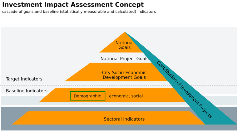
Figure. System of indicators used in assessing the impact of investment projects on socio-economic development
Demographic SED indicators are basic indicators characterizing the state and development of the city, they are initial for calculating social (provision with socio-economic objects, real disposable income of the population) and economic development (consumption volumes, payroll funds, and local taxes) indicators. The logical links of demographic indicators included in the Model with other basic SED indicators are presented in the figure.

Figure. Relationships of the Model’s demographic indicators with other basic SED indicators
The Model allows, based on an incomplete series of retrospective values, to form both long-term (decades) and medium-term (years) forecast values, as well as to restore missing ones and correct “anomalous” values in the retrospective period.
Main tasks of the demographic model: 1. Determination of stable trend coefficients describing changes in indicators over time. 2. Restoration of retrospective values of indicators using interpolation to improve the quality of municipal statistics. 3. Calculation of the baseline (inertial) forecast of demographic indicators for the calculation period. 4. Calculation of scenario-based demographic indicators, taking into account possible “man-made” events (investment project, expansion of territories, catastrophic phenomena) occurring at one time (“jump”) changing or not changing the trend at the choice of the Model user.
7.1.2 Main parameters, indicators, and notation
The Model allows for forecast calculations for the following demographic indicators:
| № | Demographic Indicator Name | Unit |
|---|---|---|
| 1 | Population | people |
| 2 | Number of births | people |
| 3 | Birth rate | ppm |
| 4 | Number of deaths | people |
| 5 | Mortality rate | ppm |
| 6 | Number of arrivals | people |
| 7 | Arrival rate | ppm |
| 8 | Number of departures | people |
| 9 | Departure rate | ppm |
| 10 | Natural increase (decrease) | people |
| 11 | Natural increase rate | ppm |
| 12 | Migration increase (decrease) | people |
| 13 | Migration increase rate | ppm |
The following notation for parameters and auxiliary indicators is used in the Model:
| № | Symbol | Name | Unit |
|---|---|---|---|
| 1 | \(t\) | Time (calendar date), year (month, day, hour) | year |
| 2 | \(N\) | Population size | people |
Actual values according to the Federal State Statistics Service (FSSS)
| № | Symbol | Name | Unit |
|---|---|---|---|
| 3 | \(N_{[20ХХ]}\) | Actual population as of January 1 of 20ХХ | people |
| 4 | \(B_{[20ХХ]}\) | Number of births in 20ХХ | people/year |
| 5 | \(D_{[20ХХ]}\) | Number of deaths in 20ХХ | people/year |
| 6 | \(E_{[20ХХ]} = B_{[20ХХ]} – D_{[20ХХ]}\) | Natural increase (decrease) in 20ХХ | people/year |
| 7 | \(I_{[20ХХ]}\) | Number of arrivals for permanent residence in 20ХХ | people/year |
| 8 | \(O_{[20ХХ]}\) | Number of departures for permanent residence in 20ХХ | people/year |
| 9 | \(M_{[20ХХ]} = I_{[20ХХ]} – O_{[20ХХ]}\) | Migration increase (decrease) in 20ХХ | people/year |
| 10 | \(∆N_{[20ХХ]} = E_{[20ХХ]} + M_{[20ХХ]}\) | Population increase (decrease) in 20ХХ | people/year |
| 11 | \(K_{Р[20ХХ]} = 2000·B_{[20ХХ]} / (N_{[20ХХ]} + N_{[20ХХ + 1]})\) | Birth rate, equal to the number of births in 20ХХ per thousand population in 20ХХ | ppm/year |
| 12 | \(K_{С[20ХХ]} = 2000·D_{[20ХХ]} / (N_{[20ХХ]} + N_{[20ХХ + 1]})\) | Mortality rate, equal to the number of deaths in 20ХХ per thousand population in 20ХХ | ppm/year |
| 13 | \(K_{Е[20ХХ]} = K_{Р[20ХХ]} – K_{С[20ХХ]}\) | Natural increase (decrease) rate | ppm/year |
| 14 | \(K_{П[20ХХ]} = 2000·I_{[20ХХ]} / (N_{[20ХХ]} + N_{[20ХХ + 1]})\) | Migration arrival rate, equal to the number of arrivals in 20ХХ per thousand population in 20ХХ | ppm/year |
| 15 | \(K_{У[20ХХ]} = 2000·O_{[20ХХ]} / (N_{[20ХХ]} + N_{[20ХХ + 1]})\) | Migration departure rate, equal to the number of departures in 20ХХ per thousand population in 20ХХ | ppm/year |
| 16 | \(K_{М[20ХХ]} = K_{П[20ХХ]} – K_{У[20ХХ]}\) | Migration increase (decrease) rate | ppm/year |
| 17 | \(K_{[20ХХ]} = K_{Е[20ХХ]} + K_{М[20ХХ]}\) | Population increase (decrease) rate | ppm/year |
Calculated values
| № | Symbol | Name | Unit |
|---|---|---|---|
| 18 | \(N(t)\) | Calculated population at time t | people |
| 19 | \(N`(t)=dN/dt\) | Rate of change in population | people/year |
| 20 | \(\nu_{B}(t)\) | Calculated birth rate coefficient at time t | 1/year |
| 21 | \(\nu_{D}(t)\) | Calculated mortality rate coefficient at time t | 1/year |
| 22 | \(B_{(20XX)}\) | Calculated number of births in 20ХХ | people/year |
| 23 | \(D_{(20XX)}\) | Calculated number of deaths in 20ХХ | people/year |
| 24 | \(E_{(20XX)} = B_{(20XX)} - D_{(20XX)}\) | Calculated natural increase (decrease) in 20ХХ | people/year |
| 25 | \(w_{I}(t)\) | Migration arrival rate at time t | people/year |
| 26 | \(w_{O}(t)\) | Migration departure rate at time t | people/year |
| 27 | \(I_{(20XX)}\) | Calculated number of arrivals in 20ХХ | people/year |
| 28 | \(O_{(20XX)}\) | Calculated number of departures in 20ХХ | people/year |
| 29 | \(M_{(20XX)} = I_{(20XX)} - O_{(20XX)}\) | Calculated migration increase (decrease) in 20ХХ | people/year |
| 30 | \(∆N_{(20XX)} = E_{(20XX)} + M_{(20XX)}\) | Calculated population increase (decrease) in 20ХХ | people/year |
Approximation errors
| № | Symbol | Name | Unit |
|---|---|---|---|
| 31 | \(\varepsilon_{N_{[20XX]}} = N_{(20XX)} - N_{[20XX]}\) | Absolute error in population as of January 1 of 20ХХ | people |
| 32 | \(\varepsilon_{B_{[20XX]}} = B_{(20XX)} - B_{[20XX]}\) | Absolute error in number of births in 20ХХ | people |
| 33 | \(\varepsilon_{D_{[20XX]}} = D_{(20XX)} - D_{[20XX]}\) | Absolute error in number of deaths in 20ХХ | people |
| 34 | \(\varepsilon_{E_{[20XX]}} = E_{(20XX)} - E_{[20XX]}\) | Absolute error in natural increase (decrease) in 20ХХ | people |
| 35 | \(\varepsilon_{I_{[20XX]}} = I_{(20XX)} - I_{[20XX]}\) | Absolute error in number of arrivals in 20ХХ | people |
| 36 | \(\varepsilon_{O_{[20XX]}} = O_{(20XX)} - O_{[20XX]}\) | Absolute error in number of departures in 20ХХ | people |
| 37 | \(\varepsilon_{M_{[20XX]}} = M_{(20XX)} - M_{[20XX]}\) | Absolute error in migration increase (decrease) in 20ХХ | people |
| 38 | \(\varepsilon_{∆N_{[20XX]}} = ∆N_{(20XX)} - ∆N_{[20XX]}\) | Absolute error in population increase (decrease) in 20ХХ | people |
Statistical estimates
| № | Symbol | Name | Unit |
|---|---|---|---|
| 39 | \(P\) | Confidence probability (taken as 90% in calculations) | % |
| 40 | \(z_{[P]}\) | Quantile corresponding to probability P, depending on the Student’s distribution | number |
| 41 | \(err(t)\) | Relative error | % |
Calculation results and forecasting
| № | Symbol | Name | Unit |
|---|---|---|---|
| 42 | \(N(t),\nu_{B}(t),\nu_{D}(t),B(t),D(t),…\) | Calculated dependencies of population (birth rate, mortality rate, number of births, deaths, etc.) on time | number |
| 43 | \(H(t)=N(t)e^{(z_{[P]}err(t))}\) | Upper bounds of the forecast with confidence probability P | number |
| 44 | \(L(t)=N(t)e^{(-z_{[P]}err(t))}\) | Lower bounds of the forecast with confidence probability P | number |
7.1.3 Used formulas and assumptions
In the most general form, the relation for population change over time \[\begin{align*} N`(t)=dN/dt, \end{align*}\] can be written as: \[\begin{align*} N`(t)=N(t)[\nu_{B}(N(t),t,S(N(t),t),Ext(t),…)-\nu_{D}(N(t),t,…)]+\\ +[w_{I}(N(t),t,S(N(t),t),Ext(t),…)-w_{O}(N(t),t,…)], (1) \end{align*}\] where \(N(t)\) – population size depending on time; birth rate \(\nu_{B}(…)\) and mortality \(\nu_{D}(…)\) coefficients, as well as migration arrival \(w_{I}(…)\) and departure \(w_{O}(…)\) rates depend on population \(N\), time \(t\), population “structure” \(S\) (age-sex, educational, national, etc.), and external conditions \(Ext\) (natural-climatic, inflation rate, dollar rate, oil price, employment, housing, epidemics, disasters).
Two levels of detailing are considered in the proposed model. Level I – for modeling and analyzing SED as a whole. Population size is calculated with subsequent division into three age groups: - younger than working age, - working age, - older than working age.
Equation (1) is reduced to (2): \[\begin{align*} N`(t)=N(t)[\nu_{B}(t)-\nu_{D}(t)]+[w_{I}(t)-w_{O}(t)], (2) \end{align*}\] where functions \(\nu_{B}(t)\), \(\nu_{D}(t)\), \(w_{I}(t)\), and \(w_{O}(t)\) include dependencies on “structure”, population size \(N\), time \(t\), and external conditions without detailing.
The main modeling problem is that the functions \(\nu_{B}(t)\), \(\nu_{D}(t)\), \(w_{I}(t)\), and \(w_{O}(t)\) are unknown, meaning the problem is “inverse”, which increases the solution complexity.
Level II – designed for detailed modeling and analysis of demographic system development. For Level II, equations (3) are built separately for each i-th age group with the addition of the “aging” process – transition from one age group to the next: \[\begin{align*} N`_{i}(t)=N_{i}(t)[\nu_{B_{i}}(t)-\nu_{D_{i}}(t)]+[w_{I_{i}}(t)-w_{O_{i}}(t)]+[u_{I_{i}}(t,S)-u_{O_{i}}(t,S)]. (3) \end{align*}\] where \(u_{I_{(i+1)}}(t,S)=u_{O_{i}}(t,S)\) are entrance/exit functions for the i-th age group. These functions are known and determined by the age-sex structure \(S\) and time \(t\).
7.1.4 Model Input Data
The input data for the Level I model are retrospective time series from FSSS (where available):
\(N_{[2000]}, N_{[2001]}, …, N_{[2023]}\) - Actual population as of January 1, people \(B_{[2000]}, B_{[2001]}, …, B_{[2022]}\) - Number of births in 20ХХ, people/year \(D_{[2000]}, D_{[2001]}, …, D_{[2022]}\) - Number of deaths in 20ХХ, people/year \(I_{[2000]}, I_{[2001]}, …, I_{[2022]}\) - Number of arrivals in 20ХХ, people/year \(O_{[2000]}, O_{[2001]}, …, O_{[2022]}\) - Number of departures in 20ХХ, people/year
7.1.5 Description of total calculation indicators
Total calculation indicators include parameters for each demographic indicator:
Year – the year characterizing the period; Period, start – the start date of the period; Period, end – the end date of the period; Fact – actual value from city statistics; Plan/Project – value of increase (decrease) caused by managed impact; Jump – binary parameter (TRUE if “Plan/Project” is entered); Calculation, average – the most expected forecast value; Calculation, upper bound – upper bound of the 90% corridor; Calculation, lower bound – lower bound of the 90% corridor.
7.1.6 Detailed description of the calculation algorithm
Step 1. Selection of functions \(\nu_{B}(t)\), \(\nu_{D}(t)\), \(w_{I}(t)\), and \(w_{O}(t)\). Four-parameter sigmoidal curves are used: \[\begin{align*} & \nu_{B}(t)=\frac{a_{B}+b_{B}(t⁄d_{B})^{c_{B}}}{1+(t⁄d_{B})^{c_{B}}}, & (4B) \\ & \nu_{D}(t)=\frac{a_{D}+b_{D}(t⁄d_{D})^{c_{D}}}{1+(t⁄d_{D})^{c_{D}}}, & (4D) \\ & w_{I}(t)=\frac{a_{I}+b_{I}(t⁄d_{I})^{c_{I}}}{1+(t⁄d_{I})^{c_{I}}}, & (4I) \\ & w_{O}(t)=\frac{a_{O}+b_{O}(t⁄d_{O})^{c_{O}}}{1+(t⁄d_{O})^{c_{O}}} & (4O) \end{align*}\] where a, b, c, d are parameters; a – value at t = 0 (January 1, 1999); b – limit value at t = \(\infty\); d – inflection date; c – determines the slope at the inflection point.
Step 2. Determination of initial parameter values using the least squares method.
Step 3.1. Solution of differential equation (2) for the retrospective period using the implicit Euler method. Equation (2) is replaced by: \[\begin{align*} &N(t_{j}+δt)(1-\frac{\nu_{B}(t_{j}+δt)δt}{2}+\frac{\nu_{D}(t_{j}+δt)δt}{2})=N(t_{j})(1+\frac{\nu_{B}(t_{j})δt}{2}-\frac{\nu_{D}(t_{j})δt}{2})+\\ &+δt(\frac{w_{I}(t_{j})+w_{I}(t_{j}+δt)}{2}-\frac{w_{O}(t_{j})+w_{O}(t_{j}+δt)}{2}). (6) \end{align*}\]
Step 3.2. Calculated values of other indicators (births, deaths, arrivals, departures) are determined.
Step 4. Error assessment. Sum of squared errors \(∑\varepsilon^{2}\) is calculated.
Step 5. Refinement of parameters a, b, c, d using the Newton method.
Step 6. Iteration of steps 3-5 until minimum error is reached.
Steps 7.1 and 7.2 Solution of equation (2) for the forecast period.
Step 8. Construction of upper and lower bounds: \[\begin{align*} &H(t)=N(t)e^{(z_{[P]}err(t))}, & (8) \\ &L(t)=N(t)e^{(-z_{[P]}err(t))}. & (9) \end{align*}\]
7.1.7 Scope of permissible application of the mathematical model
The model is suitable for population forecasting during natural and gradual development. It cannot predict sudden changes (wars, disasters) or administrative changes (territory expansion).
7.1.8 Accuracy assessment of mathematical models
Retrospective data shows high accuracy (up to 0.18% for population).
Population size, people
| City | Forecast for 2020* | Fact | Deviation |
|---|---|---|---|
| Voronezh | 1,057,863 | 1,058,261 | -0.04% |
| Krasnodar | 939,856 | 932,629 | 0.77% |
| Ufa | 1,128,730 | 1,128,787 | -0.01% |
| Arkhangelsk | 346,861 | 346,979 | -0.03% |
| Yuzhno-Sakhalinsk | 202,908 | 200,636 | 1.13% |
* forecast based on 2000–2019 data.