7.4 Model for assessing the financial performance of an investment project
7.4.1 Purpose of the model
The model for assessing the financial performance of investment projects (hereinafter - the Model) is intended for a preliminary, non-detailed assessment of the economic efficiency of investments made in a specific industry of a specific city.
The result of the Model calculations can be used to estimate socio-economic effects using the model for “Assessing the impact of an investment project on the socio-economic development of a city.”
7.4.2 Basic form of the model
The basic form of the model is the financial flow equation, calculated as follows:
\[ CF=R-C-E-I \ \ (1) \]
where:
- \(CF\) - net cash flow;
- \(R\) - revenue;
- \(C\) - cost of sales;
- \(E\) - commercial, administrative, and other expenses;
- \(I\) - investments.
The basic equation is used to estimate the expected financial flow of an investment project specified by the user and the components included in the financial flow. The estimate of the expected financial flow is then used to calculate derivative (synthetic) indicators characterizing the financial efficiency of the investment project.
The components of the financial flow are determined based on:
- user-specified values of the investment volume \(I\), the industry and the city where the project is implemented, as well as auxiliary financial and economic indicators;
- established ratios of investment volumes and basic financial and economic indicators of enterprises in the corresponding city and industry.
The estimation of the established investment volumes and basic financial and economic indicators is carried out using regression models applied to sets of accounting data of the corresponding city and industry.
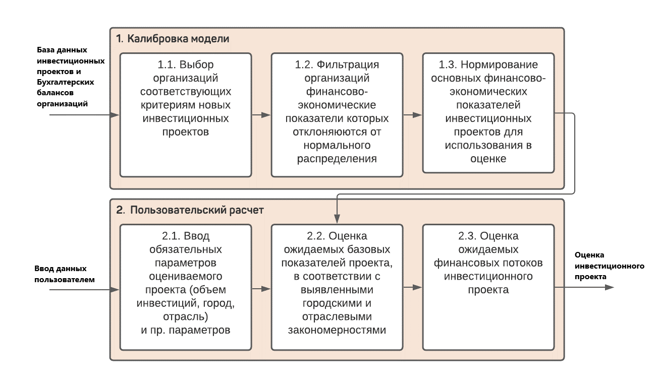
General scheme of calculations according to the Model
7.4.3 Calculation procedure
7.4.3.1 Formation of the organization sample
Selection from the total population of accounting reports was made according to the following criteria: - Organizations started activities in 2011 or later. This criterion allows selecting only relatively new organizations. - Organizations have non-zero positive values of revenue, fixed and current assets, and payroll. - Organizations have existed for 5 or more years, i.e., the sample includes organizations that have carried out their activities for a sufficiently long time.
7.4.3.2 Outlier removal
Accounting data sometimes contains dimensional errors or anomalous values. Outlier removal was performed using the following formula: \[ q 25_{i}-1.5 I Q R_{i}<X_{i}<q 75_{i}+1.5 I Q R_{i} \ \ (2) \]
where: \(X_{i}\) - indicators to be checked for outliers (\(i\) - indicator index). The list of indicators includes: - Revenue divided by the sum of cost of sales, commercial and administrative expenses; - Ratio of current assets to fixed assets; - Ratio of current assets to revenue. \(q 25_{i}\) and \(q 75_{i}\) - corresponding 25% and 75% quantiles of the distribution; \(I Q R_{i}\) - interquartile range, defined as \(I Q R_{i}= q 75_{i}-q 25_{i}\).
After the outlier removal, the total number of accounting reports used for the model was about 60,000.
7.4.3.3 Model parameter estimation
Model parameters were estimated using several methods: - Generalized Bayesian inference model with random effects, where the parameters of the posterior distribution were determined by the MCMC (Markov Chain Monte Carlo) numerical algorithm; - Generalized regression model with random effects, where the dependency parameters were determined by the maximum likelihood method using the quasi-Newton Broyden-Fletcher-Goldfarb-Shanno (BFGS) numerical algorithm.
7.4.3.4 User input of initial model parameters
The input of parameters by the user is accompanied by a check for compliance with reference information (cities and industries) and a check for possible exceeding of the investment volume value over the investment potential calculated for the current year.
7.4.3.5 Estimation of basic financial and economic indicators
K - Ratio of current assets to the total amount of assets
In accordance with the definition of \(K\):
\[ K=\frac{C A}{C A+F A} \ \ (3) \]
The indicator is estimated based on Bayesian inference by the formula:
\[ \begin{gathered} K=\beta_{0}+\beta_{1} \log (I)+\beta_{2} \text { type }_{\text {org }}+\beta_{3} \text { type }_{\text {rep }}+ eff_{city} + eff_{industry}\\ K \sim \operatorname{Beta}(C A, F A) \end{gathered} \ \ (4) \]
where: - \(I\) - investment volume; - \(\operatorname{Beta}(C A, F A)\) - Beta distribution for the ratio of current assets \(CA\) to total assets \(FA\); - \(type_{org}\) - influence of the organization type (state-owned or private); - \(type_{rep}\) - influence of the report type; - \(eff_{city}\) - random effect for the city; - \(eff_{industry}\) - random effect for the industry; - \(\beta_{j}\) - model coefficients.
R - Revenue
The indicator is estimated based on Bayesian inference by the formula:
\[ \begin{gathered} R \sim \operatorname{Gamma}(\mu, \lambda) \\ \log (\mu)=\eta \\ \eta=\beta_{0}+\beta_{1} \log (C A)+\beta_{2} \log (I)+\beta_{3} \text { type }_{\text {org }}+\beta_{4} \text { type }_{\text {rep }} + eff_{city} + eff_{industry} \end{gathered} \ \ (5) \]
where: - \(Gamma(\mu, \lambda)\) - prior Gamma distribution for revenue; - \(\mu\) - Gamma distribution parameter for the expected value shift; - \(\lambda\) - Gamma distribution parameter for scaling; - \(\log (\mu)\) - link function for \(\eta\) - auxiliary parameter; - \(\beta_{j}\) - model coefficients.
C - Cost of sales
The indicator is estimated based on Bayesian inference by the formula:
\[ \begin{gathered} C \sim \operatorname{Gamma}(\mu, \lambda) \\ \log (\mu)=\eta \\ \eta=\beta_{0}+\beta_{1} \log (R)+\beta_{2} \text { type }_{\text {org }}+\beta_{3} \text { type }_{\text {rep }} + eff_{city} + eff_{industry} \end{gathered} \ \ (6) \]
E - Commercial and administrative expenses
The indicator is estimated based on Bayesian inference by the formula:
\[ \begin{gathered} \mathrm{E} \sim \operatorname{Gamma}(\mu, \lambda) \\ \log (\mu)=\eta \\ \eta=\beta_{0}+\beta_{1} \log (R)+\beta_{2} \log (C A)+\beta_{3} type_{org}+\beta_{4}type_{rep} + eff_{city} + eff_{industry } \end{gathered} \ \ (7) \]
S - Payroll
Payroll is a component of the cost of sales and is estimated based on the cost estimate. The indicator is estimated using generalized regression:
\[ \begin{gathered} \log (S)=\beta_{0}+\beta_{1} \log (C A)+ \beta_{2} \log (F A)+ \beta_{3} \log (C)+\beta_{4} \log (C A) +\\ + \beta_{5} \log (\mathrm{K}) + \beta_{6}\left(E \mid \text { type }_{\text {rep }}\right)+ eff_{city} + eff_{industry}\\ \log (S) \sim N(\mu, \sigma) \end{gathered} \ \ (8) \]
Q - Average number of personnel
The indicator is estimated based on generalized regression:
\[ \begin{gathered} Q \sim \operatorname{Gamma}(\mu, \lambda) \\ \log (\mu)=\eta \\ \eta=\beta_{0}+\beta_{1} \log (S)+\beta_{2} \log (F A)+\beta_{3} \log (K)+\beta_{4} \log (C A) +\\ +\beta_{5} \log (\mathrm{K})+\beta_{6}\left(E \mid \text { type }_{\text {rep }}\right)+\beta_{7} \log (R) + eff_{city} + eff_{industry} \end{gathered} \ \ (9) \]
T - Investment phase duration
The indicator is estimated based on generalized regression:
\[ \begin{gathered} T \sim \operatorname{Gamma}(\mu, \lambda) \\ \log (\mu)=\eta \\ \eta=\beta_{0}+\beta_{1} \log (I)+\beta_{2} \text { year }+\beta_{3} type_{org } + eff_{city} + eff_{industry} \end{gathered} \ \ (10) \]
7.4.3.6 Estimation of the depreciation period for fixed assets
Based on Rosstat data on the volumes of accumulated fixed assets and accrued depreciation by industry, the asset depreciation period is estimated:
\[ T_{i}^{r u}=\frac{F A_{i}^{r u}}{A_{i}^{r u}} \ \ (11) \]
where: - \(T_{i}^{ru}\) - depreciation period for industry \(i\); - \(FA_{i}^{ru}\) - all-Russian volume of assets in industry \(i\); - \(A_{i}^{ru}\) - all-Russian volume of accrued depreciation in industry \(i\).
7.4.3.7 Cash flow estimation
In estimating the financial and economic indicators of an investment project, the following assumptions are used: - Investments are distributed evenly throughout the project’s investment phase; - Revenue from sales does not take into account indirect taxes, excises, or revenue from other activities; - EBITDA = R - C + A - E; - Profit tax - 20%; - Property tax - 2% taking into account depreciation; - Cash flows are calculated in current prices without using a deflator; - The key rate of the Central Bank of the Russian Federation is used as the risk-free rate for discounting cash flows and calculating NPV and DPP; - Internal rate of return (IRR) and net present value (NPV) are calculated for total investment capital (equity and debt); - A 20% VAT tax deduction is implied for investments in fixed assets.
7.4.3.8 Discounted Cash Flow (DCF)
\[ D C F=\frac{C F_{t}}{(1+i)^{t}} \ \ (12) \]
where: - \(CF_{t}\) - net cash flow; - \(i\) - discount rate (CB key rate); - \(t\) - year number.
7.4.3.10 Internal Rate of Return (IRR)
\[ \sum_{t=0}^{T} \frac{C F_{t}}{(1+I R R)^{t}}=0 \ \ (14) \]
7.4.4 Description of model input variables
The input variables consist of three blocks:
Block 1 – Financial and economic indicators of the sample of investment projects.
| No | Notation | Description | Unit |
|---|---|---|---|
| 1 | R | Revenue | mln rub |
| 2 | C | Cost of sales | mln rub |
| 3 | E | Commercial and administrative expenses | mln rub |
| 4 | S | Payroll | mln rub |
| 5 | Q | Average number of personnel | people |
| 6 | T | Investment phase duration | years |
| 7 | EBITDA | Earnings before interest, taxes, depreciation, and amortization | mln rub |
| 8 | A | Depreciation | mln rub |
Block 2 – Indicators mandatory for user input.
| No | Interface Name | Symbol | System Name | Explanation |
|---|---|---|---|---|
| 1 | Investments | I | set_invstmnt | In rubles |
| 2 | Industry | industry | set_okved | 2-digit OKVED code |
| 3 | City | city | set_oktmo | 5-digit OKTMO code |
Block 3 – Additional indicators.
| No | Interface Name | System Name | Explanation |
|---|---|---|---|
| 1 | Current assets share | set_asst_rt | Default is null (unknown) |
| 2 | Loan rate | loan_rate | Default is CB average rate |
| 3 | Risk-free rate | risk_free_rate | Default is CB key rate |
| 4 | Debt share | loan_part | Default is 0.8 |
7.4.5 Data sources for variable sets
- Accounting reports of organizations (about 60,000 reports);
- Data on investment projects (about 56,000 projects) from various sources: FAIP, RAIP, external databases, investment programs.
- Federal statistics from Rosstat.
7.4.6 Description of model result
Output data are divided into two blocks: - Block 4 – Main values of resulting indicators (IRR, NPV, PP, PI, staff size, etc.). - Block 5 – Time series for cash flow charts (Investments, Revenue, Payroll, EBITDA, etc.).